Reversible reactions and equilibrium state
Some chemical reactions do not go to completion: they can proceed in both directions. They are called reversible and written with a double arrow: A + B ⇌ C + D
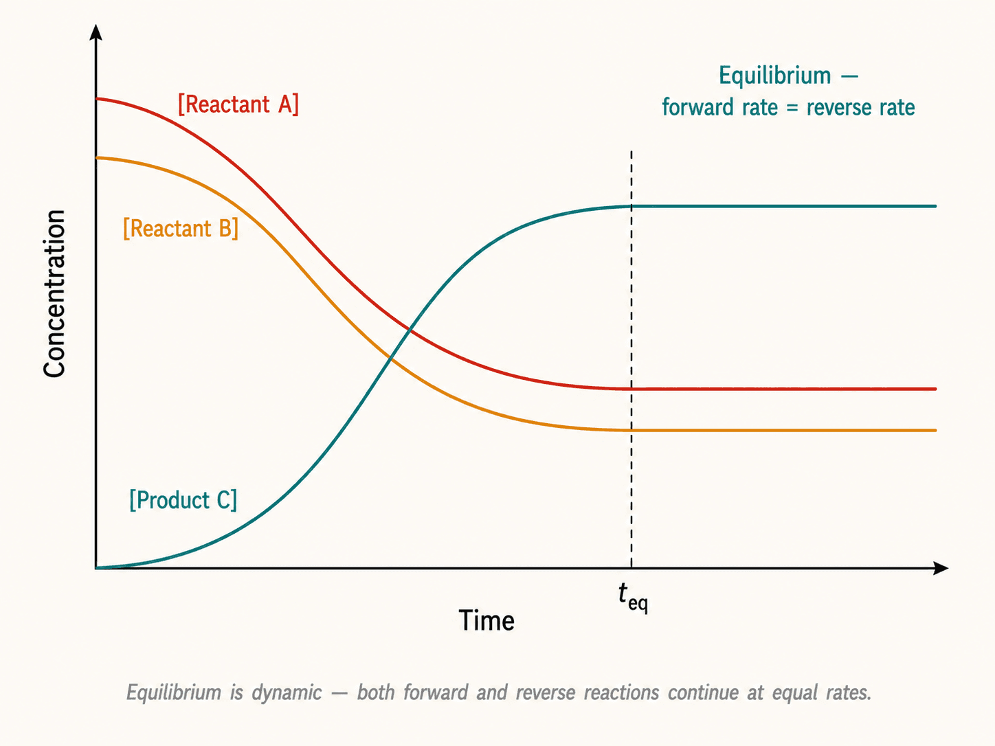
The equilibrium state is reached when the rates of the forward and reverse reactions are equal. Concentrations no longer change macroscopically, but the equilibrium is dynamic at the molecular level.
Example: synthesis of hydrogen iodide from hydrogen and iodine: H₂(g) + I₂(g) ⇌ 2 HI(g)
At high temperature, a H₂/I₂ mixture does not convert completely to HI — an equilibrium is established.
Reaction quotient Q
For the reaction a A + b B ⇌ c C + d D, the reaction quotient Q is defined at any instant by: Q = [C]ᶜ · [D]ᵈ / ([A]ᵃ · [B]ᵇ)
Q is dimensionless (concentrations divided by the standard concentration c° = 1 mol·L⁻¹). For gases, partial pressures divided by p° = 1 bar are used.
Q characterises the state of the system at any point in the reaction, not only at equilibrium.
Equilibrium constant K
At equilibrium, Q takes a unique, constant value (at a given temperature): the equilibrium constant K. K = [C]ᶜeq · [D]ᵈeq / ([A]ᵃeq · [B]ᵇeq)
K depends only on temperature (not on initial concentrations, pressure, or catalysts).
- K >> 1: equilibrium strongly shifted towards products (near-complete reaction).
- K << 1: equilibrium strongly shifted towards reactants (barely any product formed).
- K ≈ 1: significant mixture of reactants and products at equilibrium.
Evolution criterion — comparing Q and K
The evolution criterion relates Q to K to predict the direction of reaction:
| Condition | Evolution |
|---|---|
| Q < K | Forward reaction (→ towards products) |
| Q = K | Equilibrium reached, no net change |
| Q > K | Reverse reaction (← towards reactants) |
This criterion is analogous to Q vs Ksp for precipitation.
Example: for H₂(g) + I₂(g) ⇌ 2 HI(g), K = 54 at 425 °C. If H₂, I₂ and HI are mixed such that Q = 10 < K = 54: the forward reaction is favoured.
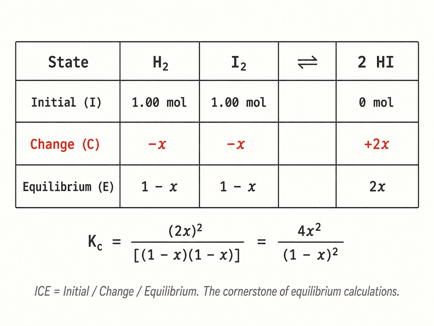
ICE table — calculating equilibrium concentrations
To calculate equilibrium concentrations, use an ICE table (Initial, Change, Equilibrium): 1. Initial concentrations [A]₀, [B]₀, [C]₀, [D]₀. 2. Stoichiometric change as a function of extent x. 3. Equilibrium concentrations as a function of x. 4. Express K as a function of x and solve (quadratic equation or approximation).
Numerical example: H₂ + I₂ ⇌ 2 HI, K = 54, [H₂]₀ = [I₂]₀ = 1 mol·L⁻¹, [HI]₀ = 0. At equilibrium: [HI] = 2x, [H₂] = [I₂] = 1 - x. K = (2x)² / (1-x)² = 54 → 2x/(1-x) = sqrt(54) ≈ 7.35 → x ≈ 0.79 mol·L⁻¹.