Rate law and reaction order
The rate law (or rate equation) expresses the reaction rate as a function of reactant concentrations: v = k [A]ⁿ [B]ᵐ
- k is the rate constant (its units depend on the overall order).
- n is the partial order with respect to A, m with respect to B.
- The overall order is n + m.
The order cannot be deduced from the balanced equation: it must be determined experimentally (stoichiometry gives the order only for elementary reactions).
Zero-order reaction
v = k (rate independent of concentration).
Integrating d[A]/dt = -k: [A] = [A]₀ - k t
The A plot is a straight line with slope -k. Half-life: t₁/₂ = [A]₀ / (2k) — depends on [A]₀.
Examples: some enzyme-saturated reactions, some surface-catalysed reactions.
First-order reaction
v = k [A].
Integrating d[A]/dt = -k [A]: [A] = [A]₀ × e^(-k t) or ln([A]) = ln([A]₀) - k t
The ln([A]) vs t plot is a straight line with slope -k. Half-life: t₁/₂ = ln(2) / k ≈ 0.693 / k — constant (independent of [A]₀).
Examples: radioactive decay, hydrolysis in dilute medium, decomposition of N₂O₅.
The constant half-life is the hallmark of first-order kinetics: after each t₁/₂, the concentration is halved.
Second-order reaction
v = k [A]².
Integrating d[A]/dt = -k [A]²: 1/[A] = 1/[A]₀ + k t
The 1/[A] vs t plot is a straight line with slope k. Half-life: t₁/₂ = 1 / (k [A]₀) — increases as [A]₀ decreases.
Examples: reaction between NO₂ and CO, decomposition of HI at high temperature.
!Comparison of [A, lnA, 1/A curves for orders 0, 1, 2](/courses/figures/rate-laws-integrated.png)
Summary of integrated rate laws
| Order | Integrated law | Linear plot | Slope | t₁/₂ |
|---|---|---|---|---|
| 0 | [A] = [A]₀ - k t | [A] vs t | -k | [A]₀/(2k) |
| 1 | ln[A] = ln[A]₀ - k t | ln[A] vs t | -k | ln2/k |
| 2 | 1/[A] = 1/[A]₀ + k t | 1/[A] vs t | k | 1/(k[A]₀) |
Experimental determination of order
Method of isolation (flooding method): if [B]₀ >> [A]₀, the concentration of B stays quasi-constant, and the rate law simplifies to: v = k' [A]ⁿ with k' = k [B]₀ᵐ (pseudo-order n with respect to A)
Repeating with different initial concentrations [A]₀ and plotting the three linear graphs (see table) identifies order n.
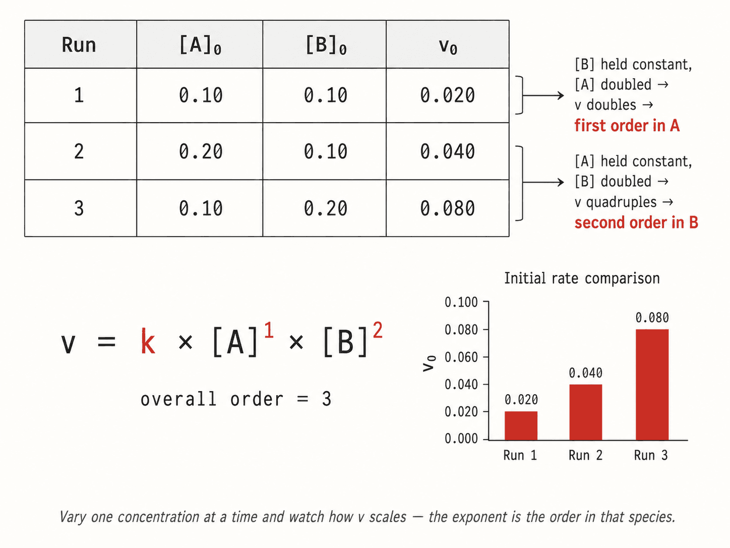
Initial rate method: measure v₀ = v(t=0) at different [A]₀: v₀ = k [A]₀ⁿ → log(v₀) = log(k) + n log([A]₀)
The slope of the log(v₀) vs log([A]₀) plot gives n directly.
Arrhenius equation and temperature dependence
The rate constant k depends on temperature via the Arrhenius equation: k = A × e^(-Ea / (R T))
- Ea: activation energy (J·mol⁻¹)
- A: pre-exponential factor (collision frequency)
- R = 8.314 J·mol⁻¹·K⁻¹, T in Kelvin
Linearised form: ln(k) = ln(A) - Ea/(R T) The ln(k) vs 1/T plot is a straight line with slope -Ea/R.