The dilution principle
Diluting a solution means lowering its concentration by increasing its volume with additional solvent. The amount of solute stays constant:
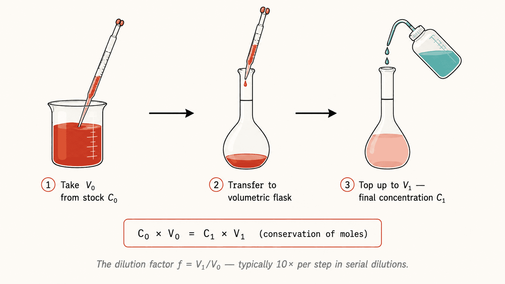
n₁ = n₂ → C₁ × V₁ = C₂ × V₂
- C₁, V₁: concentration and volume of the stock solution (before dilution).
- C₂, V₂: concentration and volume of the working solution (after dilution).
The dilution factor F is defined as:
F = C₁ / C₂ = V₂ / V₁
A dilution factor of 10 means the working solution is 10 times less concentrated than the stock.
Dilution protocol using a volumetric flask
1. Calculate the volume V₁ to pipette: V₁ = C₂ × V₂ / C₁. 2. Pipette V₁ with a volumetric pipette (±0.01 mL precision for a 10 mL pipette). 3. Transfer into a volumetric flask of volume V₂. 4. Fill to the graduation mark with solvent. 5. Stopper and mix.
Example: prepare 100 mL of HCl at C₂ = 0.050 mol/L from a stock solution at C₁ = 1.00 mol/L.
V₁ = (0.050 × 0.100) / 1.00 = 5.0 × 10⁻³ L = 5.0 mL
Pipette 5.0 mL, transfer to a 100 mL flask, fill to the mark with water.
Serial dilutions
When a very high dilution factor is needed (e.g. 10⁶), a single step is impractical because the volume to pipette would be too small to measure accurately. Instead, use serial dilutions.
Example: cascade of 1:10 dilutions (F = 10 at each step): - Step 1: C₁ → C₁/10 - Step 2: C₁/10 → C₁/100 - Step 3: C₁/100 → C₁/1000
After k steps of factor F: C_k = C₁ / Fᵏ.
Serial dilutions are common in biology (bacterial counts, immunological assays) and analytical chemistry.
Experimental verification by spectrophotometry
Beer-Lambert law relates the absorbance A of a colored solution to its concentration C:
A = ε × l × C
where ε is the molar extinction coefficient (L·mol⁻¹·cm⁻¹) and l is the optical path length (in cm). A calibration curve (series of standard solutions with known concentrations) gives the straight line A = f(C) and allows the concentration of an unknown to be read off. This is the most direct experimental check of a dilution.
| Dilution step | C (mol/L) | Measured absorbance A |
|---|---|---|
| Stock solution | 1.00 × 10⁻³ | 0.850 |
| F = 2 | 5.00 × 10⁻⁴ | 0.425 |
| F = 5 | 2.00 × 10⁻⁴ | 0.170 |
| F = 10 | 1.00 × 10⁻⁴ | 0.085 |